Basics

Detector & statistics in a nutshell

1. Statistical data analysis in a nutshell
   
2. Probability
   
3. Probability Distributions
   
4. Cumulative Distributions
   
5. Expectation Values
   
6. Functions of random variables
   
7. Specific Probability Distributions
   
   
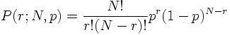
   a) BINOMIAL DISTRIBUTION
   Suppose there are two distinct outcomes of an experiment ('Kopf oder Zahl') with probabilities P(Kopf)=p, P(Zahl)=1-p and we repeat the experiment N times.
   The probability to obtain r times 'Kopf' is then given by: The mean value and variance for the binomial distribution read
   
   b) POISSON DISTRIBUTION
   If in the binomial distribution the probability of a single event becomes small and the number of trials becomes large so that μ=Np remains finite then the binomial distribution approaches a Poisson distribution which is described by one single parameter μ: The parameter μ(=Np) has the meaning of the mean value and the standard deviation at the same time.
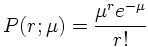
   Example: Radioactive Cs(137) nuclei have a half-life of 27 years. The decay probability per unit time for a single nucleus is then λ=ln2/27 years ≈ 8.2 10^-10 1/s. In e.g. 1 μg Cs(137) we have N=10¹⁵ nuclei (= trials). Therefore we expect μ=N λ ≈ 8.2 10⁵ decays/s and the number of observed events is distributed according to a Poissonian distribution with parameter μ. Similar arguments apply to particle scattering.
   
   c) GAUSSIAN DISTRIBUTION AND CENTRAL LIMIT THEOREM
   The Gaussian distribution for a continuous random variable x is characterized by two variables which represent the mean value and the variance of the distribution:
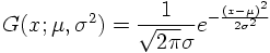
   The Gaussian distribution plays a central role in statistical data analysis due to the
   'CENTRAL LIMIT THEOREM':
   If x_i are random variables with p.d.f.'s f_i(x_i), mean values μ_i and finite variances σ_i² then the sum s=Σ_i x_i for large i is a random variable with Gaussian p.d.f. G(s;s₀,σ²) with mean s₀ = Σ_i μ_i and variance σ² = Σ_i σ_i².
   Consequences:
   a) In the limit of large μ the Poisson distribution becomes a Gaussian distribution.
   b) If a measurement is influenced by a sum of many random errors of similar size the result of the measurement is distributed according to a Gaussian distribution.
   
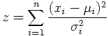
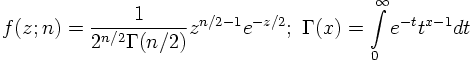
   d) χ² DISTRIBUTION
   The χ² distribution derives its importance from the fact that a sum of squares of independent Gaussian distributed random variables divided by their variances are χ²-distributed: where the parameter n is called the 'number of degrees of freedom'. The function Γ(x) is the generalisation of the factorial: The mean and the variance of the χ² distribution is n and 2n, respectively. The χ² distribution can be used in tests of goodness-of-fit in least squares fits.
   
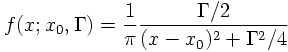
   e) BREIT-WIGNER DISTRIBUTION
   If a particle is unstable, i.e. its lifetime is finite, its energy (mass) x has a not one well-defined value but is spread according to a Breit-Wigner distribution Please note that the mean value of the Breit-Wigner distribution is not defined in the strict sense. Please note also that the variance and higher moments of the Breit-Wigner distribution are divergent as well. Nevertheless, the parameter x₀ describes the peak position and the parameter Γ describes the full-width of the peak at half maximum.
   
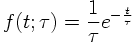
   f) EXPONENTIAL DISTRIBUTION
   The proper decay times t for unstable particles with lifetime τ are distributed according to the p.d.f.: The mean value and the standard deviation are given by the lifetime parameter τ.
   
   g) UNIFORM DISTRIBTUION
   A very important p.d.f. for practical purposes is the uniform p.d.f.:
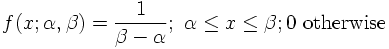
   The mean value and variance for the uniform distribution are A widely used application of the uniform distribution is the generation of pseudo-random numbers according to arbitrary p.d.f.'s f(x) using Monte Carlo techniques. One of these methods is called the transformation method and is based on the following fact:
   Starting from a random variable x with p.d.f. f(x) we define a new random variable y=F(x), given by the cumulative distribution of f(x). Independent of f(x) the new variable y is uniformly distributed between 0 and 1!
   
   
8. Parameter Estimation from Data
   
9. Statistical Tests
   
10. Basic detector concepts
    
11. Problems