So far models for random processes have been considered, that is a p.d.f. for a random variable x depending on one or more parameters θ. With the p.d.f. known and a certain parameter value of θ chosen the probability to find the variable x in a given interval can then be calculated. In the following statistical data analysis, also called statistical inference, is considered, that is, some set of data x has been measureed and the aim is to estimate the underlying parameter θ from the measured data x.
a) Maximum Likelihood Method
A p.d.f. f(x|θ) in the random variable x is considered which depends on the (a-priori unknown) parameter θ and a set of n measurements x=(x1, ..., xn) has been measured. As the n measurements are independent the probability to observe exactly this set of measurement if the true parameter value is θ is given by

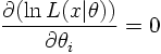
The best estimation of the parameter θ is then given by the maximum of the likelihood function (Maximum Likelihood Method) resulting in the most likely value for the parameter θ. To find the Maximum Likelihood we have to solve dL/dθ=0 or, often more conveniently,
In the large sample limit (n large) the likelihood is a Gaussian function. In this case the interval [θest-σ,θest+σ] covers the true value of the parameter θ with confidence 68 percent. In other words: if the experiment were repeated many times the interval constructed from the likelihood function in this way would cover the true value in 68 percent of the experiments.
b) Curve fitting (Least squares fits or χ² fits)
In the limit of large statistics the Maximum Likelihood Method is identical to the method of least squares. Suppose n data points yi with errors σi depending on the data points xi have been measureed and y is supposed to be a function of x, y=f(x;θ), depending on m a-priori unknown parameters θ=(θ1,...,θm). The aim is then to estimate θ from the data. For this purpose the following function is considered
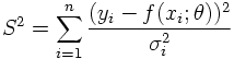

If the hypothesis (y=f(x;θ)) is correct, and if the errors are Gaussian distributed and well-estimated, the function S² is distributed according to a χ² distribution with n-m degrees of freedom. If the χ² value found in the fit is much larger than its expectation value this is a hint that either the hypothesis of the fitting model is wrong or that the errors are underestimated. In this sense the χ² is a test statistic as explained in more detail in the next section.
EXAMPLE:
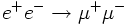
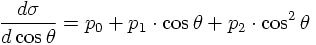
In the following a simple fit example using (ROOT) is discussed. As it will be seen later on the differential cross section for the process
* For this purpose start './epem2mupmum' and choose the energy, number of events and 'costheta' as option.
* The distribution will be shown inside a ROOT Canvas. Save the result as PCal.C and leave the program with Ctrl-C.
* Start ROOT by typing 'root'.
* Type '.x PCal.C' which will plot the cosθ histogram (the histogram object is called 'CosTheta_py').
* Afterwards type '.x simplefit'. The result of the fit is overlaid and the parameter values and uncertainties are printed. The value of 'FCN' (=S2) is the value of χ² in the minimum. As an additional information the script provides the covariance matrix of the fit parameters.