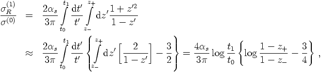
There are two ways to sum the leading logarithms, an elegant one and a brute-force one. Here the second appraoch will be chosen, resulting in explicitly summing the leading logarithms. As an example case, of course again our prime example, ee→ qqg is chosen again.
LIGHT-CONE VARIABLES
Let us start by introducing light-cone variables. They are defined in the following way:- Take any two vectors, in our case p2 and p3 and define a common (z-) axis, its spatial component points in the direction of the sum of the two vectors.
- Define transverse components of each of these vectors to be taken w.r.t. this axis, see the
figure below.
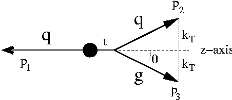
- There are two other directions, called the "+"-and the "-"-direction. The two vectors are completely determined by these two components given by (E± pz).


USING LIGHT-CONE VARIABLES: LEADING LOG APPROXIMATION
The light-cone variables introduced above are now used to rewrite the matrix element for ee→qqg in terms of z=z2+ and t:

- In most cases, the bounds of the z-integration depend on the actual value of t'. There is a simple reason for this. In principle, the treatment here does not take into account recoil effects. However, as soon as the notion of a resolution parameter is introduced, the invariant mass t' of the decaying parton/produced qaurk-gluon system together with this resolution parameter implies some conditions on the z parameter. This will be elucidated later.
- Also, as we have seen before, the coupling constant is running and one has to make a choice for the relevant scale. This choice will, of course, depend on the kinematics of the splitting, i.e. on t' and z'. In fact, it has turned out that the transverse momentum in fact is the best choice for this. In any case, α would be inside the integration.
SUMMING LEADING LOGS
Rather than trying to sum the emerging logs now by employing theoretical arguments, let us analyse and interpret the structure of the expression above. Simple considerations tell us that the 1/t' term looks like the propagator of a massless particle - in fact, it is the propagator of the "decaying" particle. Similarly, the splitting function is a local approximation of the full amplitude, projected on the piece where a specified quark line decays into quark and gluon. In other words, it is something like a "decay amplitude" squared.Let us formulate this in yet another fashion: in fact there are two quark lines (quark and antiquark) that could emit a gluon. In the language of Feynman diagrams, these two diagrams/amplitudes would have to be summed before squaring them. By going to the soft and collinear limit (collinear w.r.t. one quark line), as done above, the effect of the other quark line vanishes and typical quantum interferences are suppressed. It should be stressed here that this interpretation is a very pictorial one, written in the language of Feynman diagrams one still has a freedom of gauging the gluon field, where specific gauges support or destroy this simple interpretation. Anyways, choosing a type of gauge called the axial gauge, one can choose a gauge vector (axis) such that there is a clear and unambigous way to tell which one of the two diagrams gave rise to the leading pole.
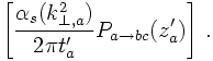
However, having at hand this interpretation of a decaying particle, it is simple to try to iterate this process of gluon emission by one of the quark lines. Including in a proper way the running of α one thus finds

In order to have maximally large logarithms it is easy to understand the various t' are ordered such that

ANGULAR ORDERING
Let us turn for a second to the case of QED radiation and consider a virtual photon splitting into an electron-positron, which in turn emits another photon, see below.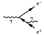

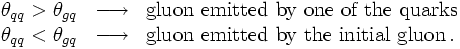
In QCD, life is a bit more complicated. This is easy to understand by just replacing the photons with gluons and the electron-positron pair by a quark-antiquark pair. The main difference here is that the net colour charge of the quark-antiquark pair differs from zero, hence they can emit the extra gluon coherently. This however can be interpreted such that the initial gluon emitted the extra gluon before splitting into a quark-antiquark pair. Taken together, in this case there are two options
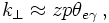
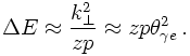
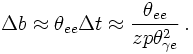
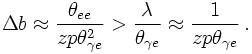
Quantum coherence is modelled best by using the opening angle or the transverse momenta of the pairs produced in parton splitting rather than using the invariant mass squared of the decaying partons. The choice of transverse momentum as the relevant scale for the splitting in the coupling constant motivates to use also transverse momenta instead of the t'. Simple calculation indeed shows that in the soft-collinear limit, the propagator term is roughly given by the transverse momentum squared. in fact, a more careful analysis of the QCD radiation pattern including the effect of quantum coherence shows that employing such an ordering in transverse momenta (rather than in masses, as above) allows to take into account not only the doubly leading logarithms but also the most relevant single logs. This is known as the modifield leading log approximation (MLLA).
RESUMMATION AND THE SUDAKOV FORM FACTOR
Let us now return to the expression above for multiple gluon emission. When replacing the virtual masses with the corresponding transverse momenta, the limits of the z-integration can easily be fixed. This allows to define the integrated splitting function, aka the branching function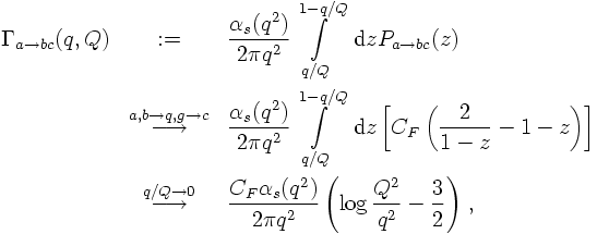
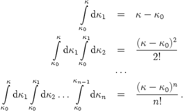
It is then simple to see that the inverse, known as the Sudakov form factor
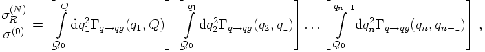
NLL JETRATES IN ee→ hadrons
Coming back to the interpretation of the Sudakov form factor it is now easy to construct expression for resummed jet rates at MLLA accuracy. For instance, the two-jet rate in ee-annihilations at the level of quarks and gluons is just given by the probability that neither the quark nor the antiquark emit a resolvable gluon. Choosing now a jet definition based on transverse momenta, like, e.g. the Durham scheme, it is clear how this connects with the Sudakov form factors: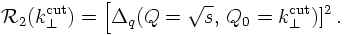

SIMULATIONS
The probabilistic interpretation of the Sudakov form factor lends itself a way to a simulation of the multiple emission pattern of QCD radiation. Such simulations have a Markovian structure - they can be set up in a recursive fashion with (up to kinematics) independent emissions. In such simulations, aka parton showers, starting from a scale Q, the next emission at scale q is recovered by equating a ratio of Sudakov form factors (exactly like the one above) with a random number. Since this ratio gives the probability for no resolvable emission between the two scales, one minus this ratio yields the probability for having an emission at q. Thus equating this ratio with a random number and solving for q yields the correct distribution of QCD radiation in terms of transverse momenta.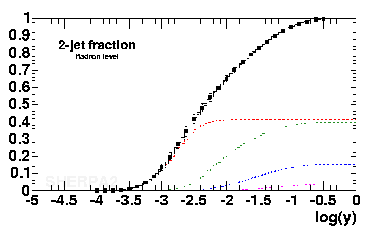 |
 |
 |
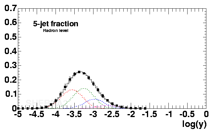 |
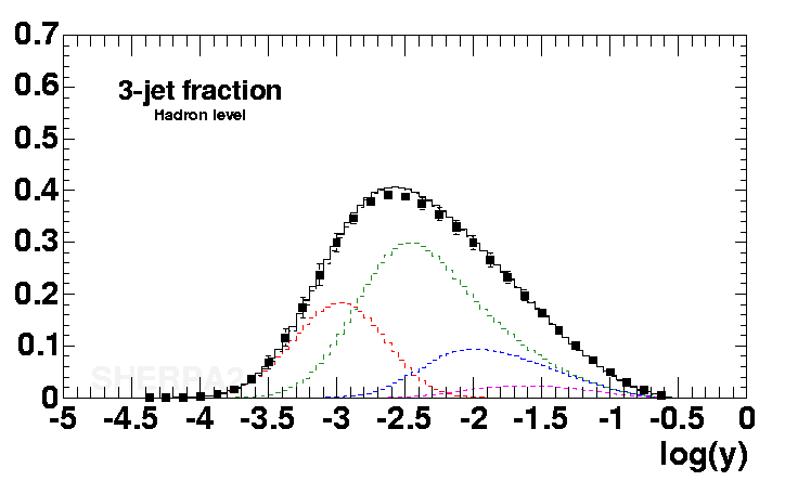
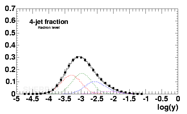
| In the plots above, y is the square of the resolution cut divided by the c.m. energy. The c.m. energy is 91.2 GeV (LEP1), thus y=0.01 corresponds to transverse momenta of 9.12 GeV, y=0.0001 corresponds to transverse momenta of 0.9 GeV. In all plots above, data (the boxes) are from LEP1, and can be found in a publication by Pfeifenschneider et al.. The black line is a simulation by Sherpa. |