QCD

Multiple gluon/parton radiation

1. e⁺e^-→ hadrons at higher orders
   

   THE DIAGRAMS AND RELEVANT PIECES OF THE AMPLITUDES

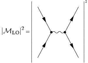
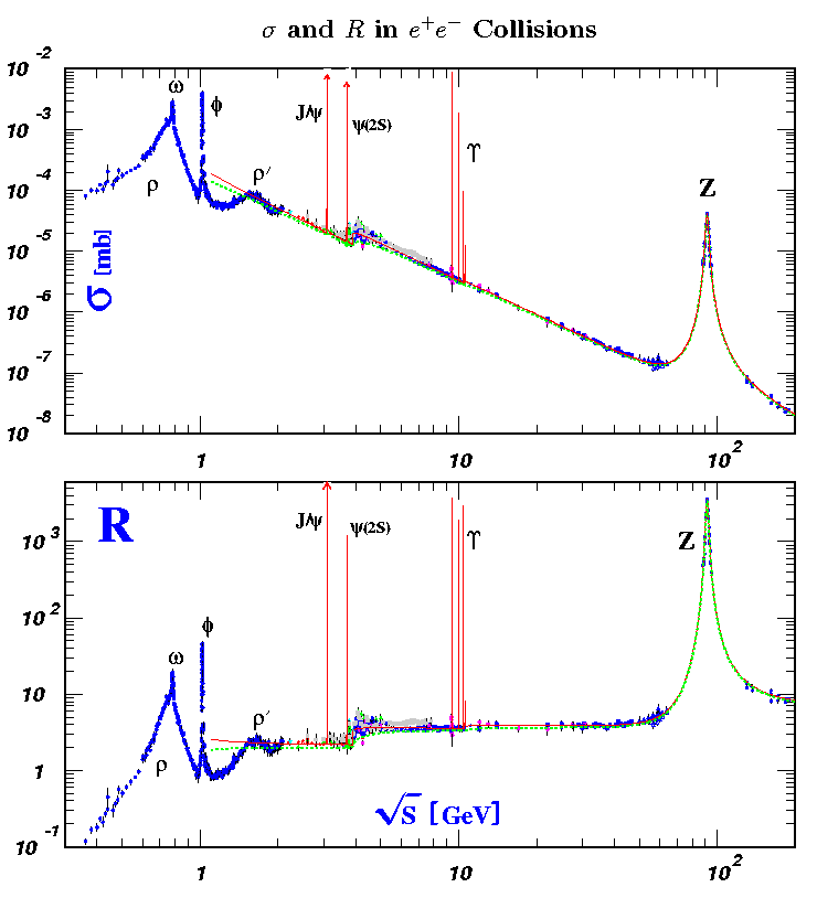
   Let us return to the total hadronic cross section in electron-positron annihilations. As has been discussed before, at leading order in perturbation theory the total cross section for the production of a massless quark-antiquark pair q reads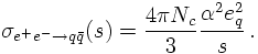 Here N_c=3 is the number of colours, s is the Mandelstam variable, i.e. the c.m. energy squared, e_q is the fractional charge of the quark in question, and α is the fine structure constant. Of course, the total hadronic cross section then is given by the sum of all quarks that are kinematically accessible, i.e with mass smaller than half of the c.m. energy of the colliding electron-positron pair. In this reasoning, and in the following, quark mass effects have been and will be neglected in both the matrix element and the phase space integration.
   When considering perturbative corrections of the first order in the strong coupling constant, two types of diagrams contribute:
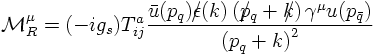
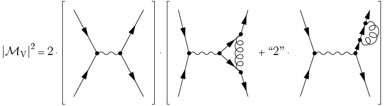
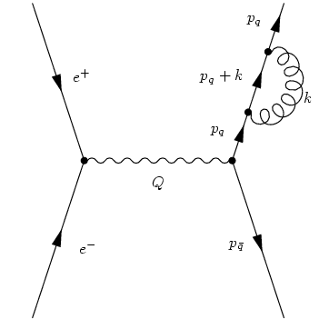
   • Corrections due to the emission of a virtual gluon, namely vertex correction and quark self energy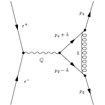
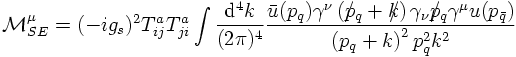
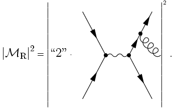
   • Also, real corrections play a role, i.e. the emission of an extra gluon:
   
   Here, two important points should be stressed:
   • Namely, first, that in all amplitudes above, only the relevant QCD part is shown, the electron current, coupling to the photon, has been ignored: it is the same as in the leading order case;
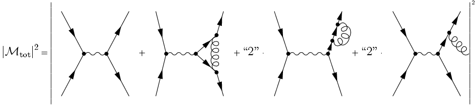
   • and that, second, the amplitudes have to be added and squared. This sounds trivial but there is some catch. The catch is easy to understand pictorially: where the "2" signify that there are two diagrams each of the corresponding kind, i.e. two self-energies and two real emission, connected to both the quark and the antiquark line, respectively. Squaring this expression, the LO contribution is readily recovered namely It is also clear that only those diagrams can be multiplied with an identical number of ingoing and outgoing legs. Therefore, at 1st order in the strong coupling constant α the virtual and the real pieces neatly separate. The virtual pieces are multiplied with the LO contribution, whereas the real pieces square directly:
   
   
   

   DIVERGENCE STRUCTURE

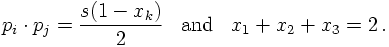
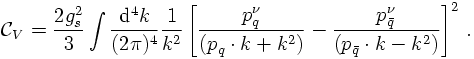
   It is clear that the virtual diagrams may contain ultraviolet divergences, that is divergences for the loop momentum k→ infinity, that need to be regularised and renormalised. However, a little bit of thought shows that both the real and the virtual diagrams also contain a new class of divergence, called infrared divergence. This new type of divergent structure appears for either k→ 0 or when the gluon momentum becomes collinear with one of the quark momenta. In order to see this better, consider first the virtual amplitudes. Applying the anticommutation rule of the γ-matrices and the E.o.M. 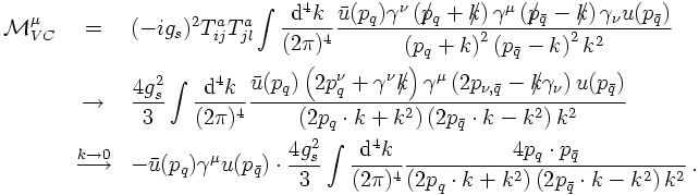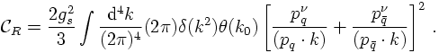for the spinors on the vertex correction term results in Clearly, at the level of approximation considered here, i.e. focusing on the most infrared-singular terms, the effect of the correction for k→ 0 results in some overall correction on the Born term. Similar reasoning also applies for the self-energy like diagrams. As a result, the terms that are most singular in the infrared region can be combined to yield Therefore the product of Born and virtual correction amplitude in this limit is proportional to the leading order amplitude squared (and thus the differential cross section) up to the loop factor
   Applying the same reasoning to the real emission pieces, a few things change a little bit: First of all, the unconstrained loop integral over k is replaced with a phase space integration over k, fixing the invariant mass of the gluon. Hence, in this case, is fixed by a δ function such that k² = 0. Second, in this case the correction term stems from both diagram pieces, cf. the scetch above. However, following the same steps as above, shows that the real correction in the infrared limit merely amounts to a corrections factor to the LO cross section, this time given by
   
   

   CANCELLATION OF INFRARED DIVERGENCES

   At this point it should be simple to see that the infrared divergencies cancel exactly. This in fact should better be the case, since in any particle physics experiment as in any other real situation, charges are accelerated leading to the emission of (electromagnetic or strong) radiation through Bremsstrahlung. This radiation is predominantly soft; taking a closer look, it turns out that the corresponding Fock state of, e.g. an electron, is populated with infinitely many photons with zero energy. In order to ensure that physical quantities such as cross sections remain finite in the presence of such soft Bremsstrahlung - as they have to, since cross sections can be measured and are finite! - these infrared divergencies have to cancel. This is the essence of two theorems, namely the Kinoshita-Lee-Nauenberg and the Bloch-Nordsieck theorems.
   At this point it is worth noting that the reasoning above in fact generalises to all orders, i.e. to arbitrarily many photons or gluons. This can be seen straightforwardly: The trick above (commuting the slashed momenta and the γ-matrices before emplyoing the E.o.M.) just needs to be repeated consecutively.
   
   

   TOTAL AND DIFFERENTIAL CROSS SECTIONS FOR ee→qq AND ee→qqg

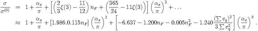
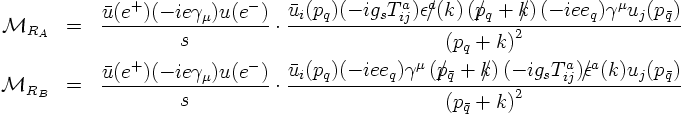
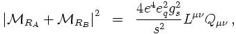
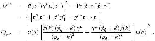
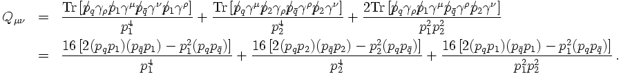
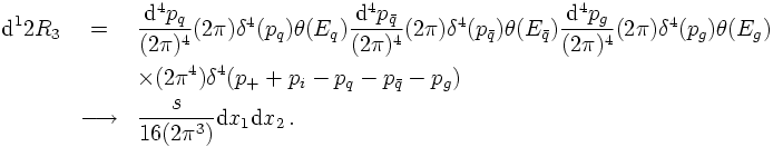
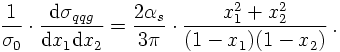
   When doing the full calculation, the total hadronic cross section reads Employing this correction, with α taken at the c.m. energy and adjusting the number of flavours appropriately, there is perfect agreement with data.
   So far, only the soft/collinear limit of real gluon emission has been dealt with. Let us now turn to a discussion of the "full truth" of extra gluon emission in quark-antiquark production in electron-positron annihilations. From the reasoning above it is clear that there are two diagrams, related to the gluon emitted by either the quark or the antiquark line. The two Feynman amplitudes read Of course they need to be summed and squared. In so doing, the lepton and the quark line can be treated independently. The total expression thus can be written as where Using completeness relations for the gluon, i.e. the sum over all polarisations, described by the product of ε and its complex conjugate, and by making suitable replacements of the p+k terms the quark piece can be written as This is a lengthy expression, that needs to be contracted with the lepton piece. In order to come to a more compact expression, it is worthwhile to introduce the dimensionless energy fractions where i=1,2,3 stands for the quark, the antiquark and the gluon, respectively. Obviously, the corresponding energies have to add up to the total c.m. energy, given by E² = s. Therefore, the sum of the three x equals 2. In addition, they satisfy the following relations In this terms, the three real contributions can be expressed as This has to be integrated over the three-particle phase space. After expressing the three (massless) momenta through the x, the three particle phase space reads Taking everything together, the differential cross section for the emission of a real gluon together with the original quark antiquark pair therefore reads This expression clearly exhibits divergencies when either of the energy fractions goes to one. The origin of this is clear, it has been noticed already before. Consider for example the case of x₁→ 1: thus for this case either one of the two energies approaches zero (the soft divergence) or the opening angle between antiquark and gluon (the collinear divergence) vanishes, resulting in a vanishing propagator term and thus in a divergence of the emission cross section. Of course, these divergences, when combined with virtual corrections vanish in the total cross section. Nevertheless, as soon as the gluon is to be resolved, i.e. as soon as we're not talking inclusive total cross sections but exclusive "gluon production" cross sections, we are left with divergencies when the resolution parameter is pushed to zero. This, however, is an unphysical concept. There is just no detector with angular or energy resolution down to zero. On top of this, the lightest QCD particle that can be measured is a hadron: the pion, with a mass of roughly 140 MeV. At least this "minimal" mass shields the soft and collinear region, after all, in order to be distinguished both the antiquark and the gluon must give rise to independent, distinct QCD particles.
   
   
2. Jets
   
3. Large logarithms and splitting functions
   
4. Resummation/exponentiation
   
5. DIS: Deep inelastic scattering and the DGLAP evolution equation
   
6. Drell-Yan processes at hadron colliders