Simple random walk and entropy
Implement a simple random walker (milk particle) on a square grid in dim dimensions. Calling the function randStep(self) in the Walker class should change the position of the walker by one unit step size in an arbitrary direction along one of the coordinate axes.
Calculate the entropy of the system from the number of micro-states. You are asked to divide the space in cubic cells with side length d and count the milk particles in each cell. Then use the formulae given in the lecture to calculate $S=k_B \ln(\Omega)$. You may set $k_B = 1$ for the purpose of this homework.
To do this, you need to:
Implement the function addPoint(self,pt) in the Grid class. It should increase the milk-particle counter of the cell in which pt is located (self.cells should be implemented as a Python dictionary with coordinates of the cell as key and the number of particles in the cell as value) and the counter for the total number of particles.
Implement the function entropy(self) in the Group class. It should use the Grid class to obtain the numbers needed to calculate $S=k_B \ln(\Omega)$ and then return $S$. Hint: The helper function logfact(x) returns $\ln(x!)$ (or a good approximation).
Milk in a cup of tea
Now we have a look at a cup of tea with a few drops of milk, in two dimensions. We want to stir the milk, so you need to impose a velocity field on the milk-particles. You also need to implement boundary conditions, i.e. the cup shouldn't leak.
In the class Environment implement the function impose_limit(self,pos) such that if a particle is further away from the center of the cup than self.radius it is put back on the radius of the cup, without changing its directions when viewed from the center of the cup (i.e. just scale the radius of the position).
The velocity field on the surface of the tea consists of two components: the circular motion and a radial component pointing to the center of the cup (the tea sinks down in the center and rises back up at the wall). The drift(self,pos) function should return the (total) velocity vector on the surface; the function phi_profile(self,r) returns the magnitude of the circular component depending on the distance r from the center of the cup, while r_profile(self,r) takes care of the radial component.
Implement the following velocity field in the drift(self,pos) function of the Environment class, making use of the phi_profile(self,r) and r_profile(self,r) functions for the tangential and radial drift components, respecively. Speeds are given in unit vector lengths per time step:
An anti-clockwise circular motion with constant speed $|v(r)|=\text{self.vphi}/\text{self.vphi_rmax}$ for $r \leq \text{self.vphi_rmax}$ and a linear decrease to zero between self.vphi_rmax and the wall.
An additional radial motion: constant radial velocity pointing towards the center of the cup with speed self.vr.
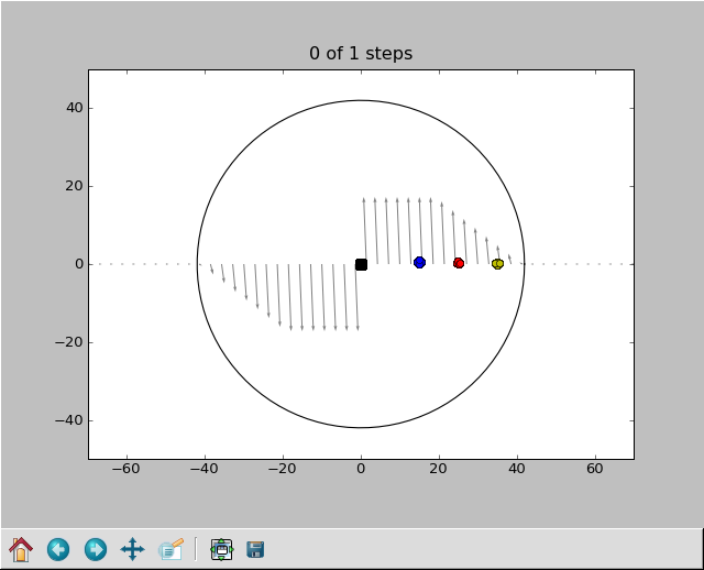
The velocity field should look like the arrows in this image: